The Xlookup Function Defaults to an Exact Match.
The formula MATCH40102040500 returns the value TRUE. Beep-boop I am a helper bot.

Xlookup Syntex Microsoft Excel Data Analyst Skill Training
XLOOKUP defaults to an exact match which is the preferred default.

. Notice that XLOOKUP doesnt require you to indicate if you want an exact or approximate match. This should be considered a step forward. If I use the XLookup function with Exact Match to locate that ID number and give me some value in a column next to it I get an NA.
The XLOOKUP match_mode parameter defaults to the exact match 0 which is not the case for the VLOOKUP HLOOKUP and MATCH functions defaulting to an approximate match. The XLOOKUP function defaults to an exact match. The search_mode parameter defines a.
The default search mode is an exact search no need to type FALSE like in the 4th argument of VLOOKUP. If I leave the cell in its. In the following figure you are looking up W25-6 from cell A4.
Please do not verify me as a solution. The full function in the function bar should read VLOOKUPC3Ingredient ListB2E1440. If Exact match is not available the function returns the next smaller item.
There are several reasons why this new XLOOKUP function is better. I dont explicitly specify the match mode exact vs. By default an exact match is performed.
No need to count columns any longer. The fourth argument for XLOOKUP allows you to specify an alternate value to display instead of NA. You do not have to enter an additional argument for it.
If you always use the exact match version of VLOOKUP you can start leaving the match_mode off of your XLOOKUP function. Similarly in the XLOOKUP function 1 works for the next larger value but in INDEX-MATCH 1 works for the next smaller value. If the look up value is not available the function returns a NA.
There is a similarity between the two functions in this aspect. You can now also lookup in a negative direction ie. If Exact match is not available then the function returns the next larger item.
It now defaults to this so you only need to flag if you dont want an exact match. It can lookup data to the right or left of the lookup values. Type False or 0 to get an exact match.
99 of my VLOOKUP formulas end in FALSE or 0 to indicate an exact match. If you have Excel 365 or Excel 2021 use XLOOKUP instead of VLOOKUP. The match behavior is controlled by the 5 th argument called match_mode.
XLOOKUP Benefit 1. The XLOOKUP function below looks up the value 53 first argument in the range B3B9 second argument. The older lookup functions default to the nearest match.
To the left for columns or upwards for rows. It allows you to provide a custom value or text if your search result is not found. If a match doesnt exist then XLOOKUP can return the closest approximate match.
Approximate in the XLOOKUP exact match example formula. However in some cases an exact match is not required. The match aspect of the XLOOKUP defaults to an exact match which is useful for text.
XLOOKUP with exact and approximate match. The difference is in what it returns if an exact. Exact Match by Default.
By default the XLOOKUP Function finds an exact match from the top of the lookup array going down ie top-down. Please pay attention that even when you choose an approximate match match_mode set to 1 or -1 the function will still search for an exact match first. XLOOKUPs new match mode allows more flexible searches.
This is because unlike VLOOKUP which defaults to an approximate match XLOOKUP defaults to an exact match. 1 Returns the Exact Match. The MATCH function searches by default for the largest value that is less than or equal to the lookup value.
The XLOOKUP function searches by default for an exact match of the lookup value. If not wanting an exact match you can now specify the previous OR the next bracket. The XLOOKUP function is easier to use and has some additional advantages.
Once it finds a match it returns the corresponding value from the return array. If youve been inserting columns in VLOOKUP you had to adapt the return column number. 2 Sheets at Once.
And thats also the reason why XLOOKUP is much more stable. You can also stop specifying false to get an exact match. The most compressed thread commented on today has 14 acronyms.
Otherwise it returns an error. In Case of Matching Wildcards. 4 acronyms in this thread.
This is also the default option-1 Returns the Exact Match. 0 Returns Exact Match. For example in the table below we have sales by person and the commissions rate they earn are in the second table.
Use the fifth argument to specify otherwise. In the XLOOKUP function -1 works for the next smaller value but in INDEX-MATCH -1 works for the next larger value. However if I manually locate that exact ID number and place the cell in edit mode and then exit the cell without taking any other step to alter the data in any way the XLookup function returns the correct result.
The REPLACE function removes all spaces from a text string except for single spaces between words. You want to look for that item in L8L35. By default the XLOOKUP function in Excel 3652021 performs an exact match.
The formula NOTORFALSEFALSETRUE will return a value of TRUE. It looks for an exact match by default. Just provide search and return columns.
The last item is looking for whether you would like to use an approximate match or an exact match. The EXACT function is not case sensitive. In almost every scenario you encounter you will want to use an exact match.
Excel Functions Xlookup

Excel Xlookup Function Won T Detect An Exact Match Until I Place The Cell In Edit Mode And Then Exit Stack Overflow
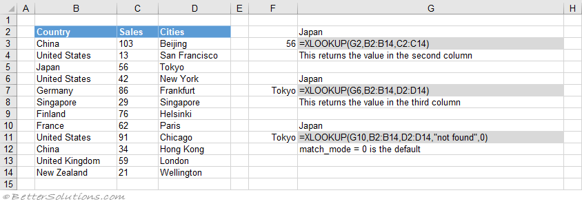
Excel Formula Xlookup Basic Exact Match Exceljet
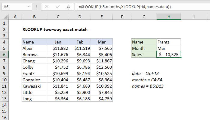
Excel Formula Xlookup Two Way Exact Match Exceljet
No comments for "The Xlookup Function Defaults to an Exact Match."
Post a Comment